
It’s widely agreed in the industry that simple byte signatures aren’t enough to reliably detect malware anymore. Instead, modern anti-virus products heavily rely on some combination of static and dynamic analysis to feed features into predictive models which determine if a particular file is malicious or not.
Until recently, we’ve been entirely focused on dynamic or behavioral analysis, rather than static or file-based analysis because we believe dynamic has the most potential long term and is better at detecting novel and unknown threats. Some time ago, we started researching and developing a static-based anti-virus feature and now we’re starting to roll it out to customers. In this post, I’m going to discuss the strengths and weaknesses of static analysis and give an overview of how we use machine learning and static feature extraction to determine if a file is malicious.
What are the Strengths and Weakness of Static Detection?
Generally, dynamic analysis is watching what a program does when it’s executed and static analysis is examining what a file looks like when it’s not running. Detecting malware using dynamic analysis involves heavily instrumenting the operating system and watching programs as they run for suspicious or malicious behaviors and stopping them (i.e. run it and see what it does). Static analysis, on the other hand, just looks at the file itself and tries to extract information about the structure and data in the file.
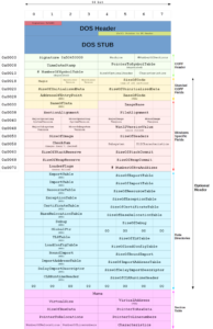
Unfortunately, many free tools exist which malware authors use to pack, encrypt, and obfuscate a file’s data and code. However, it’s not possible to entirely encrypt an executable’s structure since it must be interpreted by the operating system. This structure is fairly easy to parse and contains information about how the program was created and how it may behave. For example, you may be able to determine when the program was compiled, what compiler was used, and what API calls it might make. You can see from the picture below the structure that Microsoft’s Portable Executable format contains a great deal of information:
One of the major benefits of static-based detection is that it can be performed before the file is executed (or pre-execution). This is obviously useful because it’s much easier to remediate malware if it’s never allowed to execute. An ounce of prevention is worth a pound of cure. A corollary of this benefit is that even corrupt and malformed executables which won’t execute can still be detected statically. Of course, any sort of detection which is mostly based on behavioral analysis will fail to detect these same samples because they don’t generate any behavior. It’s questionable if these types of files should even be considered malicious. Even still, there may be some value in detecting and removing malware which can’t actually harm you simply because it brings peace of mind and suits existing policies and procedures.
Even if malware can execute, it’s often the case that it is impotent because vital command and control (C&C) servers are quickly taken down after initial discovery. Many malware families rely on instructions or additional payloads from C&C servers to operate and thus actually behave maliciously. As with corrupt files which fail to execute, it can be argued that these files are only nominally malicious, but removing them is still desirable because it removes a potential source of uncertainty to the standard operating environment.
As for disadvantages of static detection, it’s more difficult to detect completely new and novel threats that are sufficiently unlike any files you’ve seen previously. One reason for this is that it’s much easier to manipulate the structure of an executable than it is to alter the behavior. Consider the behavior of ransomware. A legitimate app can be modified in a way such that it doesn’t appear to be malicious, yet it acts like a ransomware. If you’re just looking at file structure, you’ll know about what functions it imports, but you won’t know if or when they’re called or in what order. Since most of the app’s code and structure is legitimate, it may be hard to detect particular file depending on the sophistication of your static analysis. However, even with simple dynamic analysis, you’ll see a program opening many files, calling cryptography functions, writing new files, and deleting existing files soon after starting. This behavior looks highly suspicious and is mostly endemic to ransomware.
In summary, the advantages of static detection are:
- can be performed pre-execution
- works on samples with dead C&C servers
- works on invalid executables
- computationally inexpensive
While the major disadvantages are:
- doesn’t reliably determine behavior
- doesn’t detect what happens in memory
- less likely to detect novel threats
- easier to develop counter-measures
Machine Learning Overview
Machine learning is a vast and ever-changing field and what I’ll be describing here is generally concerned with how machine learning applies to the anti-virus industry and specifically how we are using it to predict if a file is malicious or benign.
Creating a predictive model starts with collecting a huge number and variety of malicious and benign files. Then, features are extracted from each file along with the file’s label (e.g. malicious or benign). Finally, the model is trained by feeding all of these features to it and allowing it to crunch the numbers and find patterns and clusters in the data. Depending on how good your hardware is, this may take many hours or days. In this way, when the features of a file with an unknown label are presented to the model, it can return a confidence score of how similar these features are to those of the malicious and benign sets.
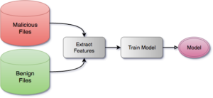
After we create the model, we can deploy it to our customers and our agent can use it to scan any new files it sees:

For various reasons which I’ll describe below, we settled on using a Random Forest for our model. Random forests are almost unreasonably effective and work decently well out of the box without much tuning, even with very large numbers of features.
To help illustrate how random forests work, I have contrived an absurd example involving feline and canine husbandry that I hope makes up for it’s lack of rigorous math with humor and pictures.
Let’s say you own a vast ranch full of cats and dogs and you’ve built a robot which will help you take care of all of them. The robot needs to be able to determine if an animal is a cat or a dog so it knows which protocol to use when treating the animal. Of course, anyone who’s owned or operated a cat knows they are special snowflakes which require slightly different handling than dogs.
Now, let’s stipulate the robot can extract the following features from an animal using various tactical and visual sensors:
- number of legs
- covered in fur
- sometimes goes outdoors
- loves you
- lives outdoors exclusively
- has sharp teeth
- sometimes wears a leash
- falls asleep in odd places
- attacks without warning
- excellent sense of smell
You’ll notice that features #1 and #2 are both always true for all animals, assuming they’re healthy and normal. These features do not add any useful information so random forests will ignore them.
To train your random forest, you’ll first need to extract the features for each animal on your bizarre ranch and record them in something like a spreadsheet:
| # | number of legs | covered in fur | sometimes goes outdoors | loves you | … |
|---|---|---|---|---|---|
| 1 | 4 | 1 | 1 | 1 | … |
| 2 | 4 | 1 | 0 | 0 | … |
| 3 | 4 | 1 | 1 | 0 | … |
| 4 | 4 | 1 | 0 | 1 | … |
| 5 | 4 | 1 | 1 | 1 | … |
And for each row of features, another spreadsheet contains the label (cat or dog) for that animal:
| # | label |
|---|---|
| 1 | dog |
| 2 | cat |
| 3 | cat |
| 4 | cat |
| 5 | dog |
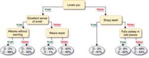
The process of training a random forest is really a process of creating many decision trees where each node in the tree represents an if-else of some feature value. In a random forest, the features for each decision tree are determined somewhat randomly, but in this example every feature is used for simplicity. As the decision tree is trained, each row of features is run through the decision tree by following all of the conditionals. The leaves of the tree contain the probabilities that a particular label would reach that particular leaf. Here’s an example decision tree of the above features. The leaves contain two probabilities one for C (cat) and one for D (dog).
One way of computing the total score is to run the features through each decision tree in the forest and average the scores together.
To complete the analogy between real life and this animal ranch, you can always invest more time in developing ways of extracting more meaningful features to improve the accuracy your model. For example, you may intuit that the following features are useful:
- likes to go outside
- learns new tricks easily
- loves you only when it’s convenient
- assumes you’ve abandoned it forever whenever you leave
Unfortunately, these features are much more complex and will require a lot of additional effort to extract. So, you keep a list of all the fancy features you’d like to have and save them for version 2.0.
Extracting and Selecting Features
We wanted to detect Windows executable malware so we started by experimenting with pefile which is a library for parsing Portable Executables. It gave us a good number of features. For example, this is the output of analyzing kernel32.dll.
We scanned each file to produce a large set of raw features. Some features had values which were strings, such as section names (.text, CODE, .bss, etc.), while others were either a floating point number (entropy), or were binary (0 or 1).
Many learning algorithms only work with features which have numeric values. If you want to use strings, you have to vectorize your input data. Vectorization converts your raw features, which may include strings, into a nice, clean, easily-machine-readable bit vector. For example, this is a list of raw features which includes entropy, file size, and strings of PE section names:
| sha256 | features |
|---|---|
| 34973274ccef6ab4dfaaf86599792fa9c3fe4689 | sect0: ‘.text’, sect1: ‘.data’, entropy: 3.1415926, size: 1234 |
| aa6c73ce643102b45ed60d462cfc8d9eb771677a | sect0: ‘CODE’, sect1: ‘.data’, entropy: 2.71828, size: 256 |
| c8fed00eb2e87f1cee8e90ebbe870c190ac3848c | sect0: ‘.bss’, sect1: ‘.text’, entropy: 1.6180339, size: 512 |
After processing, this is the bit vector or feature matrix:
| sha256 | sect0_.text | sect0_CODE | sect0_.bss | sect1_.data | sect1_.text | entropy | size |
|---|---|---|---|---|---|---|---|
| 34973274ccef6ab4dfaaf86599792fa9c3fe4689 | 1 | 0 | 0 | 1 | 0 | 3.1415926 | 1234 |
| aa6c73ce643102b45ed60d462cfc8d9eb771677a | 0 | 1 | 0 | 1 | 0 | 2.71828 | 256 |
| c8fed00eb2e87f1cee8e90ebbe870c190ac3848c | 0 | 0 | 1 | 0 | 1 | 1.6180339 | 512 |
Each column represents a feature or a dimension. As you can see, the original number of raw features (excluding sha256) is only sect0, sect1, entropy and size, but the number of dimensions in the feature matrix is 7. In our case, we started with about 60,000 different raw features but when vectorized the number of dimensions grew to over 1,000,000.
Many machine learning and clustering algorithms work by determining spacial relationships between data points. Having many dimensions increases the noise and complexity of the data set (you try and visualize 1,000,000 dimensions!) and it’s usually good to reduce the number of dimensions using principal component analysis (PCA), feature agglomeration, and feature selection. These steps can improve both training time and predictive accuracy because there’s less noise in the training data.
PCA works by projecting a high dimensional graph of the features on to a lower dimensional space in a way that preserves the most information possible for a given number of dimensions. For a much better and more detailed explanation, check out Kernel tricks and nonlinear dimensionality reduction via RBF kernel PCA. Feature agglomeration works by clustering highly correlated features together. Feature selection is often done by training a model with all features and scoring the usefulness of each feature. In subsequent trainings, you can drop features which are not deemed useful enough. All of these require a lot of experimentation and tuning to get right.
We experimented with PCA and feature agglomeration but we got the best test results by only using only feature selection. Before performing feature selection, we removed all invariant features or features that were the same for every sample. Then, we calculated the ANOVA F-value for each feature and dropped all features below some threshold. We determined the optimal threshold by inspecting the F-values and finding that a sizable number of features were above a certain level and most features were far below that level. In the end, we had a feature matrix with about 31,000 features.
As we continue to develop our static detection engine, we’ll have to continue to collect new malicious and benign samples. As our sample set grows, so to does training time. Many files are highly similar, so it will eventually become important for us to experiment with different feature selection methods that can be used for quick and accurate sample clustering. By using clustering, we’ll be able to limit the size of our training set without negatively affecting sample diversity. We want the most diverse set possible so that our model remains accurate even when used on files we have never seen before.
Choosing and Tuning a Model
We experimented with many different models for the original proof of concept. Because of the high number of dimensions, or perhaps of limitations of the library some other mysterious reason we couldn’t fathom, models which worked by determining decision boundaries on the vector space such as Linear SVM and Multi-layer Perceptron (MLP) neural networks performed badly. Eventually, we settled on decision trees even though I fought very hard to avoid using decision trees because I thought they were boring and not cool and I wanted to use something hip and flashy that sounded smart when I talked about it to my friends. But despite this, we went with decision tree based models and eventually settled on random forest which is just an ensemble of decision trees.
After some initial promising results with random forests, we needed to determine the best hyper parameters for training. The parameters we focused most of our attention on are:
- number of estimators (decision trees)
- quality criterion
- maximum features per split
- minimum samples per split
- maximum tree depth
- out of bag scoring
It’s impossible to know a priori the best way to tune a learning model. The only way to know for sure is by trying every permutation of certain parameters. This technique is called grid searching. In our case, we simply gave a range for each of the above parameters for building a random forest and ran a grid search for a few days. Each iteration of the grid search trained a random forest using all of the input data from our sample corpus and then did a fast, 3 fold cross validation and recorded the accuracy. Then, we plotted the results to see how well the features performed at different values and to predict how one feature might be better if we continued tuning it beyond what we initially set as the bounds of the grid search. Here’s what one of the graphs looked like:
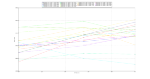
The y-axis is model accuracy and the x-axis is the number of estimators. If you have very good eyesight or you expand the image, you can see that the green circle line performs the best. This line represents max_features of 0.3, min_sample_split of 1, and oob_score of True. At around 255 estimators, it performed the best, but as the number of estimators was increased, other parameters eventually overtook and eventually out-performed it. We eventually settled on the orange octagon (max_features=0.3, min_samples_split=4, oob_score=False).
In case you’re curious, here is the code for generating the above graph: graph_gridsearch.py.
There is already ample research on machine learning for use in the anti-virus industry. Reviewing existing literature helped me understand which features and models were most likely to work well and, most importantly, build some intuition as to why they would work.
However, in my opinion, there are two major caveats to keep in mind when reading academic studies: sample selection and test scores vs real world scores. With regards to sample selection, many studies used fewer than 100,000 samples and there often isn’t a discussion of the diversity or freshness of the sample set. I don’t think this is due to ignorance or laziness but it’s a lot of extra work and the consequences of a small, stale sample set are subtle and not felt strongly until you arm your model with the ability to delete files and deploy it on thousands of machines in the real world. Similarly, many papers cited test results with model accuracies exceeding 99.9% accuracy–meaning false negatives and false positives together were less than 0.1%. When evaluating our own models with the standard 10 fold cross validation we also had similar scores. However, if we downloaded several thousand new malicious and benign files which had not been trained on, our model accuracy would drop by 0.5-5%. This means you shouldn’t be overly impressed by cross validation scores and you must also test against samples from various sources not in the training set. We solved this issue by simply increasing our training set size and diversity.
Conclusion
I hope you’ve learned something reading this and that you have a better understanding of machine learning in general and how it applies to the anti-virus industry. I believe that this new static-based detection feature nicely compliments our dynamic engine and our customers will be better protected with it.